Employing some fancier data science skills this week, I aim to create a Null Sampling distribution using the “College tuition, diversity, and pay” data set. I will be analyzing the differences in cost/tuition between public and private schools. I will filter out the data in order to make a fair comparison between the two categories (e.g. schools in the same region), then compare the difference between their costs.
Here is a citation for my data set:
National Center for Education Statistics. 2024. Tuition Tracker. Integrated Postsecondary Education Data System (IPEDS). Retrieved from https://www.tuitiontracker.org
“The Tuition Tracker dataset uses raw data from the U.S. Department of Education’s IPEDS to analyze tuition trends across U.S.-based, degree-granting institutions. Projected prices are based on historical trends from 2012-13 to 2022-23, adjusted using the compound annual growth rate and sticker prices. Net price projections consider average discount rates by income level.”
My research questions involve seeing whether tuition rates are higher for private universities than for public universities. My null hypothesis claim: Tuition rates do not differ between public and private universities.
I am only interested in the total cost for students attending schools in-state, in California. This way, the cost-of-living is fairly looked at (since comparing California schools with Maine schools, for example, would not be fair).
# A tibble: 239 × 4
   name                                    state_code type    in_state_tuition
   <chr>                                   <chr>      <chr>              <dbl>
 1 Allan Hancock College                   CA         Public              1418
 2 Alliant International University        CA         Private            18000
 3 American Academy of Dramatic Arts: West CA         Private            35160
 4 American Jewish University              CA         Private            31826
 5 American River College                  CA         Public              1416
 6 Antelope Valley College                 CA         Public              1420
 7 Antioch University Los Angeles          CA         Private            20670
 8 Antioch University Santa Barbara        CA         Private            22575
 9 Art Center College of Design            CA         Private            43416
10 Azusa Pacific University                CA         Private            38880
# ℹ 229 more rows
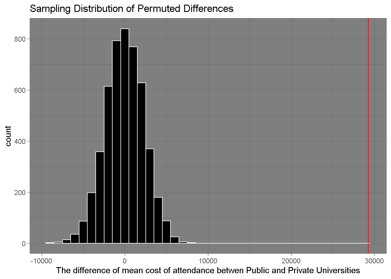
# My function to simulate a random sampling of school's in-state tuition# My function to simulate a random sampling of school's in-state tuition# averageavg_cost <- CA_schools |>group_by(type) |>summarize(avg_cost =mean(in_state_tuition))avg_diff <- CA_schools |>group_by(type) |>summarize(avg_cost =mean(in_state_tuition)) |>summarize(ave_diff =diff(avg_cost))avg_diff_val <-abs(avg_diff$ave_diff[1])# medianmed_cost <- CA_schools |>group_by(type) |>summarize(median_cost =median(in_state_tuition))med_diff <- CA_schools |>group_by(type) |>summarize(median_cost =median(in_state_tuition)) |>summarize(median_diff =diff(median_cost))med_diff_val <-abs(med_diff$median_diff[1])# average cost codeperm_data <-function(rep, data){ CA_schools |>select(type, in_state_tuition) |>mutate(perm_type =sample(type)) |>group_by(perm_type) |> dplyr::summarize(perm_cost =mean(in_state_tuition, na.rm =TRUE)) |>summarize(diff_perm =diff(perm_cost), rep = rep)}#map(1:10, perm_data, data = avg_diff) |> # list_rbind()set.seed(65)# 1000 iterationsnum_exper <-5000simulated_differences <-map(1:num_exper, perm_data, data = avg_diff) |>list_rbind()simulated_differences |>data.frame() |>ggplot(aes(x = diff_perm)) +geom_histogram(binwidth =1000, fill ="black", color ="white") +geom_vline(xintercept = avg_diff_val, color ="red") +labs(x ="The difference of mean cost of attendance betwen Public and Private Universities",title ="Sampling Distribution of Permuted Differences") +theme_dark()
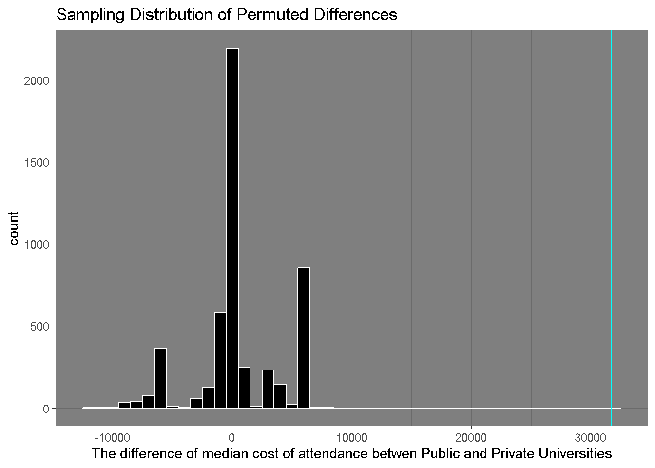
median_simulated_differences |>data.frame() |>ggplot(aes(x = median_diff_perm)) +geom_histogram(binwidth =1000, fill ="black", color ="white") +geom_vline(xintercept = med_diff_val, color ="cyan") +labs(x ="The difference of median cost of attendance betwen Public and Private Universities",title ="Sampling Distribution of Permuted Differences") +theme_dark()
This plot shows us the results from randomly shuffling the labels between public and private universities, and then measuring their mean difference.
From these data, the observed differences seem to be consistent with the distribution of differences in the null sampling distribution. This holds true for the median cost of attendance as well.
There is very strong evidence to reject the null hypothesis - our p-value is zero!
We can claim that the tuition rates are higher for private universities than for public universities (p-value = 0).
We achieved this result by filtering for California schools, and then calculating the average mean between private and public schools in California. We then shuffled their labels, and ran this over 1000 iterations, and found that there is strong evidence for the null hypothesis in this case.